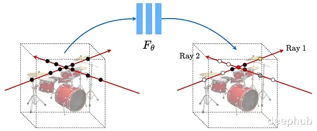
NeRF（Neural Radiance Fields，神经辐射场）的核心思路是用一个全连接网络表示三维场景。输入是5D向量空间坐标(x, y, z)加上视角方向(θ, φ)，输出则是该点的颜色和体积密度。训练的数据则是同一物体从不同角度拍摄的若干张照片。

通常情况下泛化能力是模型的追求目标，需要在大量不同样本上训练以避免过拟合。但NeRF恰恰相反，它只在单一场景的多个视角上训练，刻意让网络"过拟合"到这个特定场景，这与传统神经网络的训练逻辑完全相反。

这样NeRF把网络训练成了某个场景的"专家"，这个专家只懂一件事，但懂得很透彻：给它任意一个新视角，它都能告诉你从那个方向看场景是什么样子，存储的不再是一堆图片，而是场景本身的隐式表示。

把5D输入向量拆开来看：空间位置(x, y, z)和观察方向(θ, φ)。

颜色（也就是辐射度）同时依赖位置和观察方向，这很好理解，因为同一个点从不同角度看可能有不同的反光效果。但密度只跟位置有关与观察方向无关。这里的假设是材质本身不会因为你换个角度看就变透明或变不透明，这个约束大幅降低了模型复杂度。

用来表示这个映射关系的是一个多层感知机（MLP）而且没有卷积层，这个MLP被有意过拟合到特定场景。

渲染流程分三步：沿每条光线采样生成3D点，用网络预测每个点的颜色和密度，最后用体积渲染把这些颜色累积成二维图像。

训练时用梯度下降最小化渲染图像与真实图像之间的差距。不过直接训练效果不好原始5D输入需要经过位置编码转换才能让网络更好地捕捉高频细节。

传统体素表示需要显式存储整个场景占用空间巨大。NeRF则把场景信息压缩在网络参数里，最终模型可以比原始图片集小很多。这是NeRF的一个关键优势。

NeRF出现之前，神经场景表示一直比不过体素、三角网格这些离散表示方法。

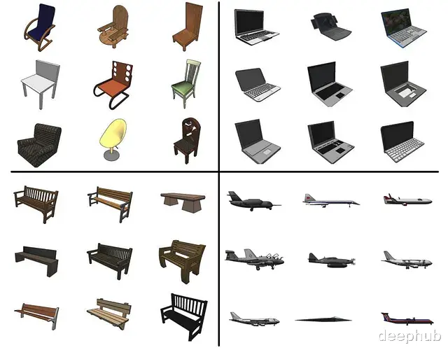
早期也有人用网络把位置坐标映射到距离函数或占用场，但只能处理ShapeNet这类合成3D数据。

arxiv:1912.07372 用3D占用场做隐式表示提出了可微渲染公式。arxiv:1906.01618的方法在每个3D点输出特征向量和颜色用循环神经网络沿光线移动来检测表面,但这些方法生成的表面往往过于平滑。

如果视角采样足够密集，光场插值技术就能生成新视角。但视角稀疏时必须用表示方法,体积方法能生成真实感强的图像但分辨率上不去。

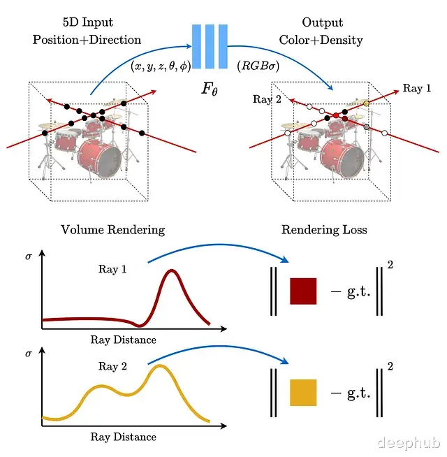
输入是位置 x = (x, y, z) 和观察方向 d = (θ, φ)，输出是颜色 c = (r, g, b) 和密度 σ。整个5D映射用MLP来近似。

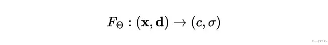
优化目标是网络权重 Θ。密度被假设为多视角一致的，颜色则同时取决于位置和观察方向。

网络结构上先用8个全连接层处理空间位置，输出密度σ和一个256维特征向量。这个特征再和观察方向拼接，再经过一个全连接层得到颜色。

光线参数化如下：

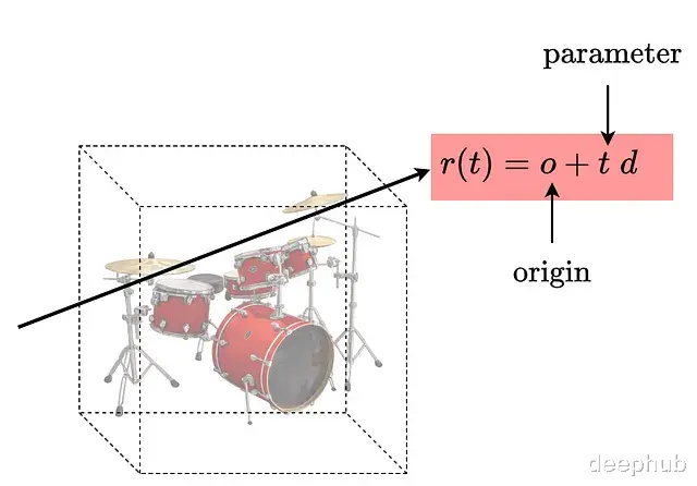
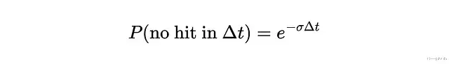
密度σ描述的是某点对光线的阻挡程度，可以理解为吸收概率。更严格地说它是光线在该点终止的微分概率。根据这个定义，光线从t传播到tₙ的透射概率可以表示为：

σ和T之间的关系可以画图来理解：

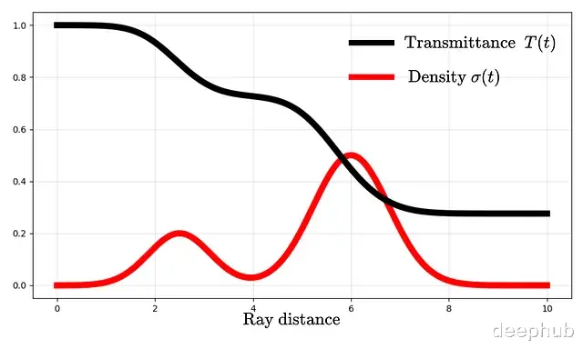
密度升高时透射率下降。一旦透射率降到零，后面的东西就完全被遮住了，也就是看不见了。

光线的期望颜色C(r)定义如下，沿光线从近到远积分：

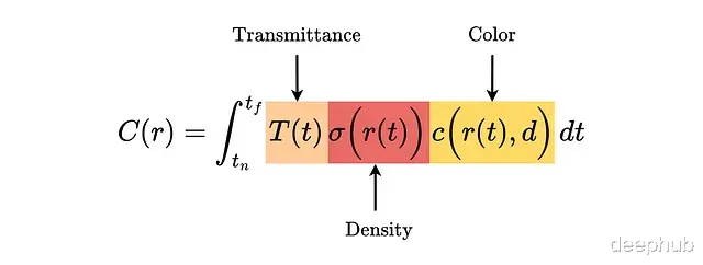
问题在于c和σ都来自神经网络这个积分没有解析解。

实际计算时用数值积分，采用分层采样策略——把积分范围分成N个区间，每个区间均匀随机抽一个点。

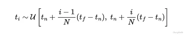
分层采样保证MLP在整个优化过程中都能在连续位置上被评估。采样点通过求积公式计算C(t)这个公式选择上考虑了可微性。跟纯随机采样比方差更低。

Tᵢ是光线存活到第i个区间之前的概率。那光线在第i个区间内终止的概率呢？可以用密度来算：

σ越大这个概率越趋近于零，再往下推导：

光线颜色可以写成：

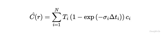
其中：

直接拿5D坐标训练MLP，高频细节渲染不出来。因为深度网络天生偏好学习低频信号，解决办法是用高频函数把输入映射到更高维空间。

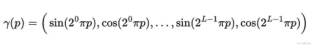
γ对每个坐标分别应用，是个确定性函数没有可学习参数。p归一化到[-1,+1]。L=4时的编码可视化：

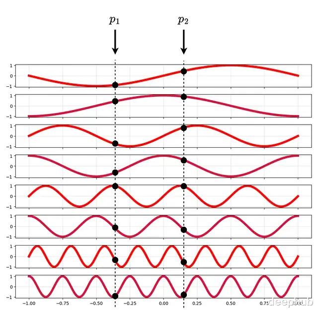
L=4时的位置编码示意

编码用的是不同频率的正弦函数。Transformer里也用类似的位置编码但目的不同——Transformer是为了让模型感知token顺序，NeRF是为了注入高频信息。

均匀采样的问题在于大量计算浪费在空旷区域。分层采样的思路是训练两个网络，一个粗糙一个精细。

先用粗糙网络采样评估一批点，再根据结果用逆变换采样在重要区域加密采样。精细网络用两组样本一起计算最终颜色。粗糙网络的颜色可以写成采样颜色的加权和。

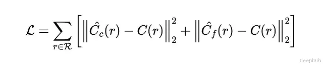
每个场景单独训练一个网络，只需要RGB图像作为训练数据。每次迭代从所有像素里采样一批光线，损失函数是粗糙和精细网络预测值与真值之间的均方误差。

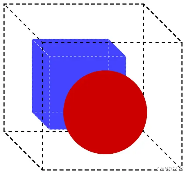
接下来从零实现NeRF架构，在一个包含蓝色立方体和红色球体的简单数据集上训练。

数据集生成代码不在本文范围内——只涉及基础几何变换没有NeRF特有的概念。

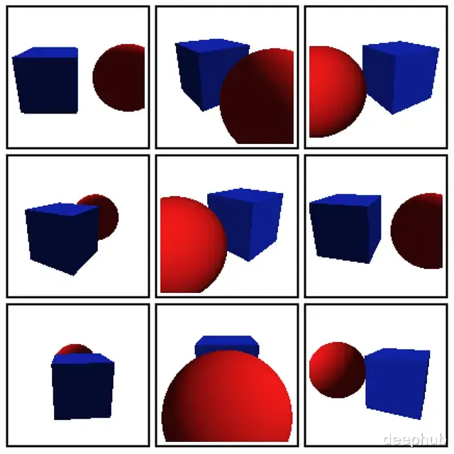
数据集里的一些渲染图像。相机矩阵和坐标也存在了JSON文件里。

先导入必要的库：

import os, json, math   import numpy as np   from PIL import Image   import torch   import torch.nn as nn   import torch.nn.functional as F

位置编码函数：

def positional_encoding(x, L):      freqs = (2.0 ** torch.arange(L, device=x.device)) * math.pi # Define the frequencies      xb = x[..., None, :] * freqs[:, None] # Multiply by the frequencies      xb = xb.reshape(*x.shape[:-1], L * 3) # Flatten the (x,y,z) coordinates      return torch.cat([torch.sin(xb), torch.cos(xb)], dim=-1)

根据相机参数生成光线：

def get_rays(H, W, camera_angle_x, c2w, device):      # assume the pinhole camera model      fx = 0.5 * W / math.tan(0.5 * camera_angle_x) # calculate the focal lengths (assume fx=fy)        # principal point of the camera or the optical center of the image.      cx = (W - 1) * 0.5      cy = (H - 1) * 0.5        i, j = torch.meshgrid(torch.arange(W, device=device),                            torch.arange(H, device=device), indexing="xy")      i, j = i.float(), j.float()            # convert pixels to normalized camera-plane coordinates      x = (i - cx) / fx      y = -(j - cy) / fx      z = -torch.ones_like(x)        # pack into 3D directions and normalize      dirs = torch.stack([x, y, z], dim=-1)      dirs = dirs / torch.norm(dirs, dim=-1, keepdim=True)            # rotate rays into world coordinates using pose matrix      R, t = c2w[:3, :3], c2w[:3, 3]      rd = dirs @ R.T      ro = t.expand_as(rd)      return ro, rd

NeRF网络结构：

class NeRF(nn.Module):      def __init__(self, L_pos=10, L_dir=4, hidden=256):          super().__init__()          # original vector is concatented with the fourier features          in_pos = 3 + 2 * L_pos * 3          in_dir = 3 + 2 * L_dir * 3            self.fc1 = nn.Linear(in_pos, hidden)          self.fc2 = nn.Linear(hidden, hidden)          self.fc3 = nn.Linear(hidden, hidden)          self.fc4 = nn.Linear(hidden, hidden)          self.fc5 = nn.Linear(hidden + in_pos, hidden)          self.fc6 = nn.Linear(hidden, hidden)          self.fc7 = nn.Linear(hidden, hidden)          self.fc8 = nn.Linear(hidden, hidden)            self.sigma = nn.Linear(hidden, 1)          self.feat = nn.Linear(hidden, hidden)            self.rgb1 = nn.Linear(hidden + in_dir, 128)          self.rgb2 = nn.Linear(128, 3)            self.L_pos, self.L_dir = L_pos, L_dir        def forward(self, x, d):          x_enc = torch.cat([x, positional_encoding(x, self.L_pos)], dim=-1)          d_enc = torch.cat([d, positional_encoding(d, self.L_dir)], dim=-1)            h = F.relu(self.fc1(x_enc))          h = F.relu(self.fc2(h))          h = F.relu(self.fc3(h))          h = F.relu(self.fc4(h))          h = torch.cat([h, x_enc], dim=-1) # skip connection          h = F.relu(self.fc5(h))          h = F.relu(self.fc6(h))          h = F.relu(self.fc7(h))          h = F.relu(self.fc8(h))            sigma = F.relu(self.sigma(h)) # density is calculated using positional information          feat = self.feat(h)            h = torch.cat([feat, d_enc], dim=-1) # add directional information for color          h = F.relu(self.rgb1(h))          rgb = torch.sigmoid(self.rgb2(h))          return rgb, sigma

渲染函数，这个是整个流程的核心：

def render_rays(model, ro, rd, near=2.0, far=6.0, N=64):      # sample along the ray      t = torch.linspace(near, far, N, device=ro.device)      pts = ro[:, None, :] + rd[:, None, :] * t[None, :, None] # r = o + td            # attach view directions to each sample      # each point knows where the ray comes from      dirs = rd[:, None, :].expand_as(pts)            # query NeRF at each point and reshape      rgb, sigma = model(pts.reshape(-1,3), dirs.reshape(-1,3))      rgb = rgb.reshape(ro.shape[0], N, 3)      sigma = sigma.reshape(ro.shape[0], N)        # compute the distance between the samples      delta = t[1:] - t[:-1]      delta = torch.cat([delta, torch.tensor([1e10], device=ro.device)])        # convert density into opacity      alpha = 1 - torch.exp(-sigma * delta)      # compute transmittance along the ray      T = torch.cumprod(torch.cat([torch.ones((ro.shape[0],1), device=ro.device),                                   1 - alpha + 1e-10], dim=-1), dim=-1)[:, :-1]        weights = T * alpha      return (weights[...,None] * rgb).sum(dim=1) # accumulate the colors

训练循环：

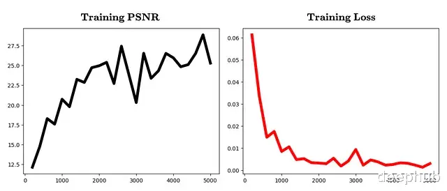
device = "cuda" if torch.cuda.is_available() else "cpu"   images, c2ws, H, W, fov = load_dataset("nerf_synth_cube_sphere")   images, c2ws = images.to(device), c2ws.to(device)    model = NeRF().to(device)   opt = torch.optim.Adam(model.parameters(), lr=5e-4)    loss_hist, psnr_hist, iters = [], [], []    for it in range(1, 5001):      idx = torch.randint(0, images.shape[0], (1,)).item()      ro, rd = get_rays(H, W, fov, c2ws[idx], device)      gt = images[idx].reshape(-1,3)        sel = torch.randint(0, ro.numel()//3, (2048,), device=device)      pred = render_rays(model, ro.reshape(-1,3)[sel], rd.reshape(-1,3)[sel])            # for simplicity, we will only implement the coarse sampling.      loss = F.mse_loss(pred, gt[sel])        opt.zero_grad()      loss.backward()      opt.step()        if it % 200 == 0:          psnr = -10 * torch.log10(loss).item()          loss_hist.append(loss.item())          psnr_hist.append(psnr)          iters.append(it)          print(f"Iter {it} | Loss {loss.item():.6f} | PSNR {psnr:.2f} dB")    torch.save(model.state_dict(), "nerf_cube_sphere_coarse.pth")    # ---- Plots ----   plt.figure()   plt.plot(iters, loss_hist, color='red', lw=5)   plt.title("Training Loss")   plt.show()    plt.figure()   plt.plot(iters, psnr_hist, color='black', lw=5)   plt.title("Training PSNR")   plt.show()

迭代次数与PSNR、损失值的变化曲线：

模型训练完成下一步是生成新视角。

look_at函数用于从指定相机位置构建位姿矩阵：

def look_at(eye):      eye = torch.tensor(eye, dtype=torch.float32) # where the camera is      target = torch.tensor([0.0, 0.0, 0.0])      up = torch.tensor([0,1,0], dtype=torch.float32) # which direction is "up" in the world        f = (target - eye); f /= torch.norm(f) # forward direction of the camera      r = torch.cross(f, up); r /= torch.norm(r) # right direction. use cross product between f and up      u = torch.cross(r, f) # true camera up direction        c2w = torch.eye(4)      c2w[:3,0], c2w[:3,1], c2w[:3,2], c2w[:3,3] = r, u, -f, eye      return c2w

推理代码：

device = "cuda" if torch.cuda.is_available() else "cpu"    with open("nerf_synth_cube_sphere/transforms.json") as f:      meta = json.load(f)    H, W, fov = meta["h"], meta["w"], meta["camera_angle_x"]    model = NeRF().to(device)   model.load_state_dict(torch.load("nerf_cube_sphere_coarse.pth", map_location=device))   model.eval()    os.makedirs("novel_views", exist_ok=True)    for i in range(120):      angle = 2 * math.pi * i / 120      eye = [4 * math.cos(angle), 1.0, 4 * math.sin(angle)]      c2w = look_at(eye).to(device)        with torch.no_grad():          ro, rd = get_rays(H, W, fov, c2w, device)          rgb = render_rays(model, ro.reshape(-1,3), rd.reshape(-1,3))        img = rgb.reshape(H, W, 3).clamp(0,1).cpu().numpy()      Image.fromarray((img*255).astype(np.uint8)).save(f"novel_views/view_{i:03d}.png")        print("Rendered view", i)

新视角渲染结果（训练集中没有这些角度）：

图中的伪影——椒盐噪声、条纹、浮动的亮点——来自空旷区域的密度估计误差。只用粗糙模型、不做精细采样的情况下这些问题会更明显。另外场景里大片空白区域也是个麻烦，模型不得不花大量计算去探索这些没什么内容的地方。

再看看深度图：

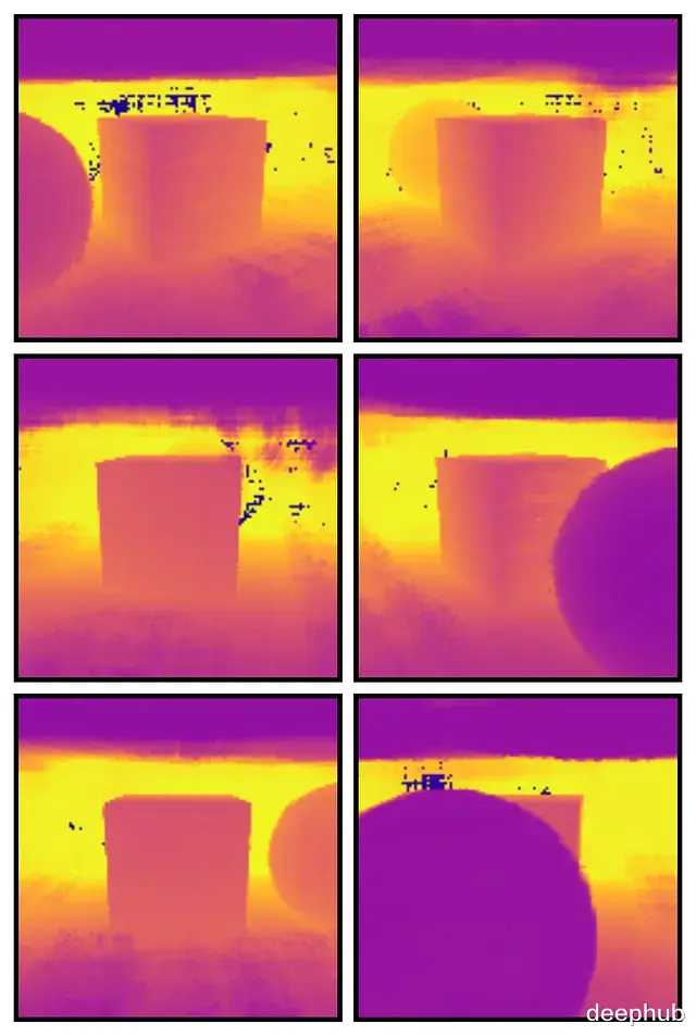
立方体的平面捕捉得相当准确没有幽灵表面。空旷区域有些斑点噪声说明虽然空白区域整体学得还行，但稀疏性还是带来了一些小误差。

参考文献

Mildenhall, B., Srinivasan, P. P., Gharbi, M., Tancik, M., Barron, J. T., Simonyan, K., Abbeel, P., & Malik, J. (2020). NeRF: Representing scenes as neural radiance fields for view synthesis.

https://avoid.overfit.cn/post/4a1b21ea7d754b81b875928c95a45856

作者：Kavishka Abeywardana